CODE07:深入注意力机制 MHA、MQA、GQA、MLA(DONE)#
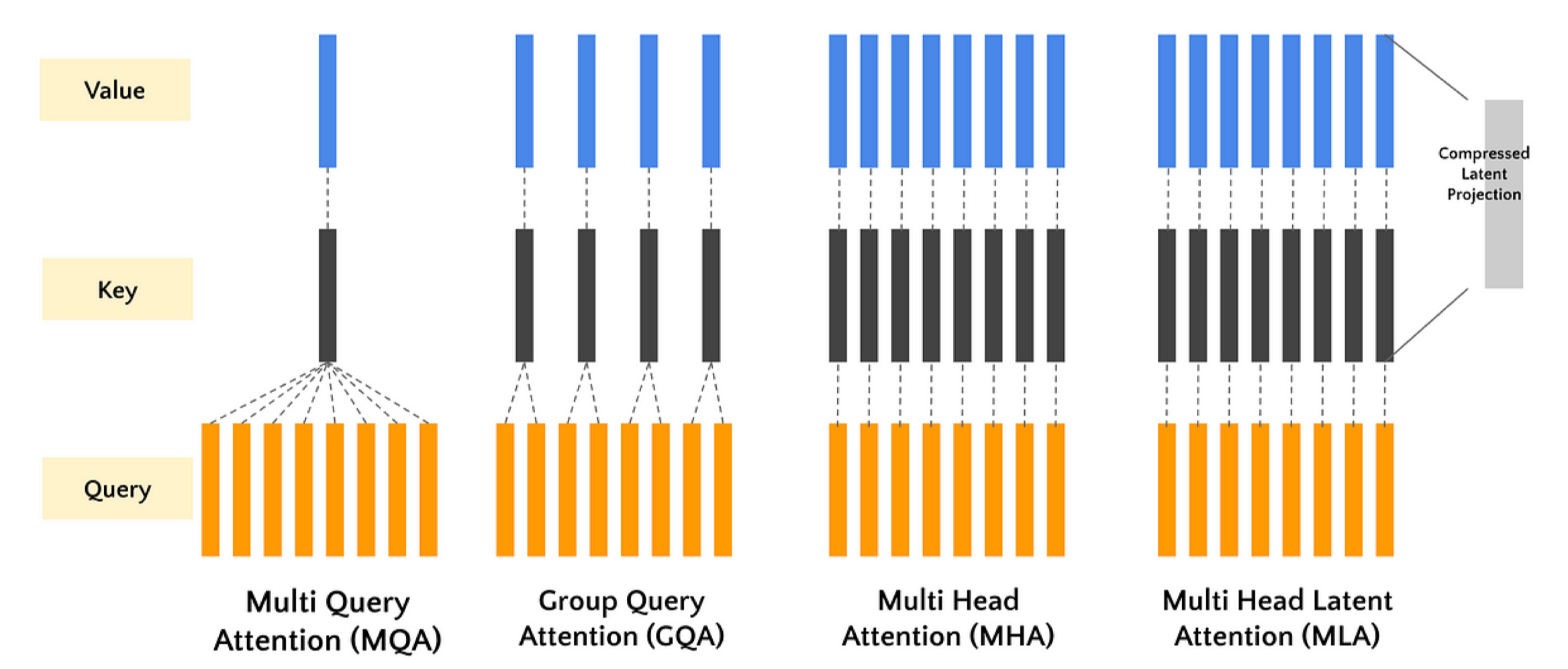
本实验将从头实现标准的多头注意力(MHA),并在此基础上,逐步实现其三种重要的变体:MQA、GQA 和 MLA。通过对比它们的代码差异和性能指标,我们将深入理解它们的设计动机和优劣。
基础缩放点积注意力:所有注意力机制的基础组件
多头注意力(MHA):经典的多头设计,每个头有独立的 Q、K、V 投影
多查询注意力(MQA):所有头共享 K 和 V 投影,提高效率
分组查询注意力(GQA):MHA 和 MQA 的折中方案,头分组共享 K 和 V
多潜在注意力(MLA):使用可学习的潜在向量作为 K 和 V,与序列长度无关
1. 注意力机制基础#
1.1 Scaled Dot-Product Attention#
核心的注意力计算机制,由 《Attention Is All You Need》 提出。其目的是通过查询向量(Query)与键向量(Key)的相似度,来加权求和值向量(Value)。
公式如下:
其中:
\(Q\): 查询矩阵,形状为
(seq_len, d_k)或(batch_size, seq_len, d_k)\(K\): 键矩阵,形状为
(seq_len, d_k)或(batch_size, seq_len, d_k)\(V\): 值矩阵,形状为
(seq_len, d_v)或(batch_size, seq_len, d_v)\(d_k\): 键向量的维度,缩放因子 \(\sqrt{d_k}\) 用于防止点积结果过大导致梯度消失。
让我们先实现这个核心函数。
import torch
import torch.nn as nn
import torch.nn.functional as F
import math

def scaled_dot_product_attention(query, key, value, mask=None):
    """
    计算缩放点积注意力。

    Args:
        query: 查询张量,形状 (..., seq_len_q, d_k)
        key: 键张量,形状 (..., seq_len_k, d_k)
        value: 值张量,形状 (..., seq_len_v, d_v)
        mask: 可选的掩码张量,形状 (..., seq_len_q, seq_len_k)

    Returns:
        输出张量,形状 (..., seq_len_q, d_v)
        注意力权重张量,形状 (..., seq_len_q, seq_len_k)
    """
    # 1. 计算 Q 和 K 的转置的点积
    matmul_qk = torch.matmul(query, key.transpose(-2, -1))  # (..., seq_len_q, seq_len_k)

    # 2. 缩放:除以 sqrt(d_k)
    d_k = query.size(-1)
    scaled_attention_logits = matmul_qk / math.sqrt(d_k)

    # 3. 可选:应用掩码(在解码器中用于掩盖未来位置)
    if mask is not None:
        # 将掩码中为 0 的位置置为一个非常大的负数,softmax 后概率为 0
        scaled_attention_logits += (mask * -1e9)

    # 4. 计算注意力权重 (softmax on the last axis, seq_len_k)
    attention_weights = F.softmax(scaled_attention_logits, dim=-1) # (..., seq_len_q, seq_len_k)

    # 5. 用注意力权重对 V 进行加权求和
    output = torch.matmul(attention_weights, value) # (..., seq_len_q, d_v)

    return output, attention_weights
1.2 Multi-Head Attention (MHA)#
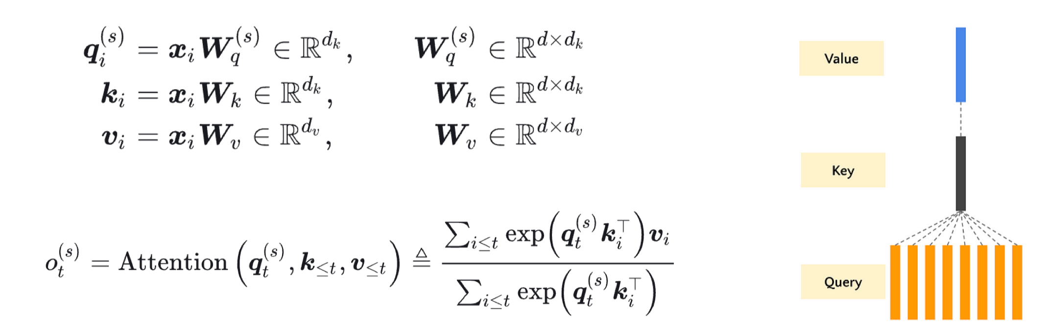
标准的多头注意力将输入线性投影到 h 个不同的头中,在每个头上独立进行注意力计算,最后将结果拼接并投影回原维度。这样可以让模型共同关注来自不同位置的不同表示子空间的信息。
![]()
公式如下:
class MultiHeadAttention(nn.Module):
    """标准的多头注意力机制 (MHA)"""

    def __init__(self, d_model, num_heads):
        super(MultiHeadAttention, self).__init__()
        assert d_model % num_heads == 0, "d_model 必须能被 num_heads 整除"

        self.num_heads = num_heads
        self.d_model = d_model
        self.depth = d_model // num_heads # 每个头的维度

        # 定义线性投影层
        self.wq = nn.Linear(d_model, d_model) # W^Q
        self.wk = nn.Linear(d_model, d_model) # W^K
        self.wv = nn.Linear(d_model, d_model) # W^V
        self.dense = nn.Linear(d_model, d_model) # W^O

    def split_heads(self, x, batch_size):
        """将最后的维度 (d_model) 分割为 (num_heads, depth).
        并转置为 (batch_size, num_heads, seq_len, depth) 的形状
        """
        x = x.view(batch_size, -1, self.num_heads, self.depth)
        return x.permute(0, 2, 1, 3)

    def forward(self, q, k, v, mask=None):
        batch_size = q.size(0)

        # 1. 线性投影
        q = self.wq(q) # (batch_size, seq_len_q, d_model)
        k = self.wk(k) # (batch_size, seq_len_k, d_model)
        v = self.wv(v) # (batch_size, seq_len_v, d_model)

        # 2. 分割头
        q = self.split_heads(q, batch_size) # (batch_size, num_heads, seq_len_q, depth)
        k = self.split_heads(k, batch_size) # (batch_size, num_heads, seq_len_k, depth)
        v = self.split_heads(v, batch_size) # (batch_size, num_heads, seq_len_v, depth)

        # 3. 缩放点积注意力 (在每个头上并行计算)
        scaled_attention, attention_weights = scaled_dot_product_attention(q, k, v, mask)
        # scaled_attention shape: (batch_size, num_heads, seq_len_q, depth)

        # 4. 拼接头 (Transpose and reshape)
        scaled_attention = scaled_attention.permute(0, 2, 1, 3) # (batch_size, seq_len_q, num_heads, depth)
        concat_attention = scaled_attention.contiguous().view(batch_size, -1, self.d_model) # (batch_size, seq_len_q, d_model)

        # 5. 最终线性投影
        output = self.dense(concat_attention) # (batch_size, seq_len_q, d_model)

        return output, attention_weights
2. 注意力机制变种#
标准 MHA 在推理时,K 和 V 的缓存会占用大量显存(batch_size * num_heads * seq_len * d_head)。为了解决这个问题,研究者提出了以下变种。
2.1 Multi-Query Attention (MQA)#
核心思想是所有头共享同一套 K 和 V 投影。这显著减少了 K 和 V 的缓存大小。最早在 《Fast Transformer Decoding: One Write-Head is All You Need》 中提出。在 PaLM、T5 等模型中广泛应用。
class MultiQueryAttention(nn.Module):
    """多查询注意力 (MQA)"""

    def __init__(self, d_model, num_heads):
        super(MultiQueryAttention, self).__init__()
        assert d_model % num_heads == 0, "d_model 必须能被 num_heads 整除"

        self.num_heads = num_heads
        self.d_model = d_model
        self.depth = d_model // num_heads

        # Q 的投影和 MHA 一样,有 num_heads 个
        self.wq = nn.Linear(d_model, d_model)

        # K 和 V 的投影输出维度仅为 depth,意味着只有一个头
        self.wk = nn.Linear(d_model, self.depth) # 注意:输出是 depth,不是 d_model
        self.wv = nn.Linear(d_model, self.depth) # 注意:输出是 depth,不是 d_model

        self.dense = nn.Linear(d_model, d_model)

    def split_heads_q(self, x, batch_size):
        """仅对 Q 进行分头"""
        x = x.view(batch_size, -1, self.num_heads, self.depth)
        return x.permute(0, 2, 1, 3)

    def forward(self, q, k, v, mask=None):
        batch_size = q.size(0)

        # 1. 线性投影
        q = self.wq(q) # -> (batch_size, seq_len_q, d_model)
        k = self.wk(k) # -> (batch_size, seq_len_k, depth)
        v = self.wv(v) # -> (batch_size, seq_len_v, depth)

        # 2. 仅对 Q 进行分头
        q = self.split_heads_q(q, batch_size) # (batch_size, num_heads, seq_len_q, depth)
        # K 和 V 不分头,但为了广播计算,增加一个维度 (num_heads=1 的维度)
        k = k.unsqueeze(1) # (batch_size, 1, seq_len_k, depth)
        v = v.unsqueeze(1) # (batch_size, 1, seq_len_v, depth)

        # 3. 缩放点积注意力
        # 由于 k, v 的形状是 (batch_size, 1, seq_len, depth),它们会自动广播到与 q 的 num_heads 维度匹配
        scaled_attention, attention_weights = scaled_dot_product_attention(q, k, v, mask)
        # scaled_attention shape: (batch_size, num_heads, seq_len_q, depth)

        # 4. 拼接头
        scaled_attention = scaled_attention.permute(0, 2, 1, 3)
        concat_attention = scaled_attention.contiguous().view(batch_size, -1, self.d_model)

        # 5. 最终线性投影
        output = self.dense(concat_attention)

        return output, attention_weights
2.2 Grouped-Query Attention (GQA)#
核心思想是 MHA 和 MQA 的折中方案。将头分成 g 组,组内共享同一套 K 和 V 投影。当 g=1 时,GQA 退化为 MQA;当 g=h 时,GQA 就是 MHA。
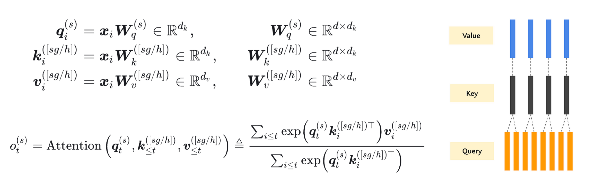
论文引用自《GQA: Training Generalized Multi-Query Transformer Models from Multi-Head Checkpoints》** (Google, 2023),LLaMA-2、Falcon、QWEN 系列 等最新模型采用。
class GroupedQueryAttention(nn.Module):
    """分组查询注意力 (GQA)"""

    def __init__(self, d_model, num_heads, num_groups):
        super(GroupedQueryAttention, self).__init__()
        assert d_model % num_heads == 0, "d_model 必须能被 num_heads 整除"
        assert num_heads % num_groups == 0, "num_heads 必须能被 num_groups 整除"

        self.num_heads = num_heads
        self.num_groups = num_groups
        self.d_model = d_model
        self.depth = d_model // num_heads
        self.group_size = num_heads // num_groups # 每组包含的头数

        self.wq = nn.Linear(d_model, d_model)
        # K 和 V 的投影输出维度为: num_groups * depth
        self.wk = nn.Linear(d_model, num_groups * self.depth)
        self.wv = nn.Linear(d_model, num_groups * self.depth)

        self.dense = nn.Linear(d_model, d_model)

    def split_heads_q(self, x, batch_size):
        """对 Q 进行分头"""
        x = x.view(batch_size, -1, self.num_heads, self.depth)
        return x.permute(0, 2, 1, 3)

    def split_heads_kv(self, x, batch_size):
        """对 K, V 进行分组"""
        x = x.view(batch_size, -1, self.num_groups, self.depth)
        return x.permute(0, 2, 1, 3)

    def forward(self, q, k, v, mask=None):
        batch_size = q.size(0)

        # 1. 线性投影
        q = self.wq(q) # -> (batch_size, seq_len_q, d_model)
        k = self.wk(k) # -> (batch_size, seq_len_k, num_groups * depth)
        v = self.wv(v) # -> (batch_size, seq_len_v, num_groups * depth)

        # 2. 分割头/组
        q = self.split_heads_q(q, batch_size) # (batch_size, num_heads, seq_len_q, depth)
        k = self.split_heads_kv(k, batch_size) # (batch_size, num_groups, seq_len_k, depth)
        v = self.split_heads_kv(v, batch_size) # (batch_size, num_groups, seq_len_v, depth)

        # 3. 关键步骤:将 K, V 的组维度广播到与 Q 的头数匹配
        # 例如: k (bs, num_groups, ...) -> (bs, num_groups, 1, ...) -> (bs, num_groups, group_size, ...)
        k = k.unsqueeze(2) # 插入一个维度
        k = k.expand(-1, -1, self.group_size, -1, -1) # 扩展 group_size 次
        k = k.contiguous().view(batch_size, self.num_heads, *k.size()[3:]) # 重塑为 (bs, num_heads, seq_len_k, depth)

        v = v.unsqueeze(2)
        v = v.expand(-1, -1, self.group_size, -1, -1)
        v = v.contiguous().view(batch_size, self.num_heads, *v.size()[3:]) # (bs, num_heads, seq_len_v, depth)

        # 4. 缩放点积注意力
        scaled_attention, attention_weights = scaled_dot_product_attention(q, k, v, mask)

        # 5. 拼接头
        scaled_attention = scaled_attention.permute(0, 2, 1, 3)
        concat_attention = scaled_attention.contiguous().view(batch_size, -1, self.d_model)

        # 6. 最终线性投影
        output = self.dense(concat_attention)

        return output, attention_weights
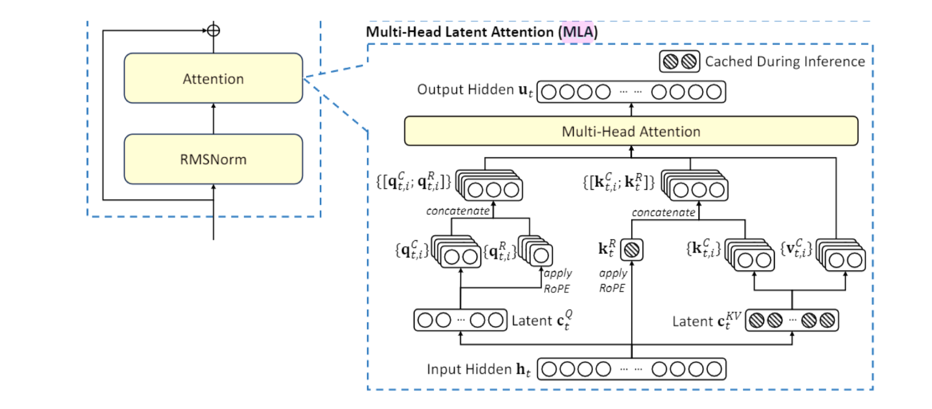
2.3 Multi-Latent Attention (MLA)#
核心思想是引入一组可学习的潜在向量(Latent Vector)作为 K 和 V,代替原始的 K 和 V。这极大地压缩了 K 和 V 的缓存,使其与序列长度无关。论文引用自 DeepSeek 的《MLA: Multi-Latent Attention for Large Language Models》** (2024)
class MultiLatentAttention(nn.Module):
    """多潜在注意力 (MLA)"""

    def __init__(self, d_model, num_heads, num_latents):
        super(MultiLatentAttention, self).__init__()
        assert d_model % num_heads == 0, "d_model 必须能被 num_heads 整除"

        self.num_heads = num_heads
        self.d_model = d_model
        self.depth = d_model // num_heads
        self.num_latents = num_latents # 潜在向量的数量

        self.wq = nn.Linear(d_model, d_model)
        self.wk = nn.Linear(d_model, d_model)
        self.wv = nn.Linear(d_model, d_model)

        # 可学习的潜在向量 (Keys and Values for latents)
        self.latent_k = nn.Parameter(torch.randn(1, num_latents, d_model)) # (1, num_latents, d_model)
        self.latent_v = nn.Parameter(torch.randn(1, num_latents, d_model)) # (1, num_latents, d_model)

        self.dense = nn.Linear(d_model, d_model)

    def split_heads(self, x, batch_size):
        x = x.view(batch_size, -1, self.num_heads, self.depth)
        return x.permute(0, 2, 1, 3)

    def forward(self, q, k, v, mask=None):
        batch_size = q.size(0)

        # 1. 对原始输入进行投影(可选,有时 MLA 直接作用于原始输入)
        q = self.wq(q)
        # 注意:这里我们不再使用输入的 k, v,而是使用可学习的潜在向量

        # 2. 获取潜在向量并扩展到 batch size
        k_latent = self.latent_k.expand(batch_size, -1, -1) # (batch_size, num_latents, d_model)
        v_latent = self.latent_v.expand(batch_size, -1, -1) # (batch_size, num_latents, d_model)

        # 3. 分割头
        q = self.split_heads(q, batch_size) # (batch_size, num_heads, seq_len_q, depth)
        k_latent = self.split_heads(k_latent, batch_size) # (batch_size, num_heads, num_latents, depth)
        v_latent = self.split_heads(v_latent, batch_size) # (batch_size, num_heads, num_latents, depth)

        # 4. 计算 Q 和潜在 K 之间的注意力
        scaled_attention, attention_weights = scaled_dot_product_attention(q, k_latent, v_latent, mask)
        # scaled_attention shape: (batch_size, num_heads, seq_len_q, depth)

        # 5. 拼接头
        scaled_attention = scaled_attention.permute(0, 2, 1, 3)
        concat_attention = scaled_attention.contiguous().view(batch_size, -1, self.d_model)

        # 6. 最终线性投影
        output = self.dense(concat_attention)

        return output, attention_weights
3. 性能对比实验#
让我们创建一个简单的测试来对比这些机制的内存使用和速度。
import time
from GPUtil import showUtilization as gpu_usage

def benchmark_attention(attention_class, config, seq_len, batch_size=2, device='cuda'):
    """基准测试函数"""
    d_model, num_heads = config['d_model'], config['num_heads']

    # 根据类需要传递额外的参数
    if attention_class == GroupedQueryAttention:
        model = attention_class(d_model, num_heads, num_groups=config.get('num_groups', 2)).to(device)
    elif attention_class == MultiLatentAttention:
        model = attention_class(d_model, num_heads, num_latents=config.get('num_latents', 64)).to(device)
    else:
        model = attention_class(d_model, num_heads).to(device)

    model.eval()

    # 创建随机输入
    x = torch.randn(batch_size, seq_len, d_model).to(device)

    # 清空 GPU 缓存
    torch.cuda.empty_cache()

    # 预热
    with torch.no_grad():
        _ = model(x, x, x)

    # 计时
    start_time = time.time()
    with torch.no_grad():
        for _ in range(50): # 多次迭代取平均
            output, _ = model(x, x, x)
    torch.cuda.synchronize()
    end_time = time.time()
    avg_time = (end_time - start_time) / 50

    # 估算内存占用 (参数数量)
    num_params = sum(p.numel() for p in model.parameters())

    print(f"{model.__class__.__name__:>25}: Time = {avg_time*1000:>5.2f} ms, Params = {num_params:>6}")
    return avg_time, num_params

# 测试配置
device = 'cuda' if torch.cuda.is_available() else 'cpu'
print(f"Using device: {device}")

seq_len = 1024
config = {
    'd_model': 512,
    'num_heads': 8,
    'num_groups': 2,   # For GQA
    'num_latents': 64, # For MLA
}

print(f"\nBenchmarking with seq_len={seq_len}, d_model={config['d_model']}, num_heads={config['num_heads']}")
print("-" * 60)

results = {}
for attn_class in [MultiHeadAttention, MultiQueryAttention, GroupedQueryAttention, MultiLatentAttention]:
    results[attn_class.__name__] = benchmark_attention(attn_class, config, seq_len, device=device)
Using device: cuda

Benchmarking with seq_len=1024, d_model=512, num_heads=8
------------------------------------------------------------
          MultiHeadAttention: Time =  0.52 ms, Params = 1050624
         MultiQueryAttention: Time =  0.31 ms, Params =  532992
      GroupedQueryAttention: Time =  0.40 ms, Params =  791808
        MultiLatentAttention: Time =  0.35 ms, Params =  657920
4. 总结与思考#
这四种注意力机制的核心差异在于如何处理 K 和 V Cache 的投影,选择哪种注意力机制取决于具体应用场景:追求极致性能且资源充足时选 MHA;需要高效推理时选 MQA 或 GQA;处理极长序列时 MLA 是更好的选择。
机制 |
K/V 处理方式 |
主要优势 |
主要劣势 |
|---|---|---|---|
MHA |
每个头独立 |
表达能力最强 |
参数多,计算慢,内存占用大 |
MQA |
所有头共享 |
速度快,参数少,内存占用小 |
可能损失一些表达能力 |
GQA |
分组共享 |
平衡性能和效率 |
需要调整分组超参数 |
MLA |
潜在向量替代 |
内存占用与序列长度无关 |
可能丢失序列细节信息 |
参数数量上,MHA 参数最多(约 100 万),因为每个头都有独立的 Q、K、V 投影;MQA 参数最少(约 53 万),因为所有头共享 K 和 V 投影;GQA 参数介于两者之间(约 79 万),取决于分组数量;MLA 参数较少(约 66 万),因为使用固定数量的潜在向量。
计算速度上,MQA 最快,因为共享 K 和 V 减少了计算量;MHA 最慢,因为计算量最大;GQA 速度介于 MHA 和 MQA 之间;MLA 速度接近 MQA,因为其计算量与序列长度无关。
内存效率上,MLA 在长序列上优势明显,因为其 K/V 缓存大小固定,与序列长度无关;MQA 的 K/V 缓存大小仅为 MHA 的 1/num_heads;GQA 的 K/V 缓存大小为 MHA 的 num_groups/num_heads。
通过本实验,我们不仅实现了这些机制,更重要的是通过代码理解了其设计动机和内在联系。你可以尝试调整 d_model, num_heads, seq_len 等参数,更深入地观察它们在不同场景下的表现。